Simulating the OLS Consistency When X and ε are Dependent - How to illustrate convergence in probability? | /en/2021/06/ols-consistency/

yihui 2022-12-17 06:26:18

Simulating the OLS Consistency When X and ε are Dependent - How to illustrate convergence in probability?

https://yihui.org/en/2021/06/ols-consistency/

3 Comments

giscus-bot 2022-12-17 06:26:19

Guest *Doruk Cengiz* @ 2021-06-10 18:33:29 originally posted:

Hi,

Fantastic and fun to read post. I love these brain teasers.

So, I have looked into it and found that (let me know if I'm mistaken), the correlation between e and x are not zero in your example. In fact, they are mostly positive, which explains the $\hat\beta$'s being slightly bigger than 2. As a matter of fact, the correlation coefficient between $\hat\beta$'s and the correlation coefficients between X and e is virtually 1.

Here is my code:

set.seed(1000)
beta_est = function(N = 10) {
 e = runif(N)
 x = (e - .5) + 100 * (e - .5)^2 + rnorm(N)
 y = 2 * x + e
 res = lm.fit(cbind(1, x), y)
 matrix(c(res$coefficients[2], cor(x,e)), ncol = 2) # the slope
}

Ns = rep(seq(10000, 15000, 200), each = 300)
bs = matrix(rep(NA, length(Ns)*2), ncol = 2)
for (i in seq_along(Ns)) {
 bs[i,] = beta_est(Ns[i])
}

par(mar = c(4, 4.5, .2, .2))
plot(
 Ns, bs[,1], cex = .6, col = 'gray',
 xlab = 'N', ylab = expression(hat(beta))
)
abline(h = 2, lwd = 2)
points(10000, 2.0014, col = 'red', cex = 2, lwd = 2)

par(mar = c(4, 4.5, .2, .2))
plot(
 Ns, bs[,2], cex = .6, col = 'gray',
 xlab = 'N', ylab = expression(hat(rho))
)
abline(h = 0, lwd = 2)

print(cor(bs[,1], bs[,2]))

giscus-bot 2022-12-17 06:26:22

Guest *Doruk Cengiz* @ 2021-06-10 18:38:36 originally posted:

In fact, if we have completely uncorrelated (but dependent) X and e's, we get hatbeta = 2. (Again, please let me know if I'm missing something):

set.seed(1000)
e = seq(-2,2, 0.0001)
x = 100 * (e)^2

d <- data.frame(e=e, x=x)

cor(d$e, d$x)
coef_error <- rep(NA,2000)

for (zz in seq_along(coef_error)){
  d$y <- 2 * d$x + d$e + rnorm(n=length(e))
  res = lm(y~x, data = d)
  coef_error[zz] <- res$coefficients[2] -2 # the slope
  
}
print(sum(coef_error<0))
print(sum(coef_error>0))
print(mean(coef_error))

yihui 2022-12-17 06:26:22

That is an interesting finding! Thank you very much! I just ran a simulation again and found that X and ε indeed became more positively correlated as N grows.

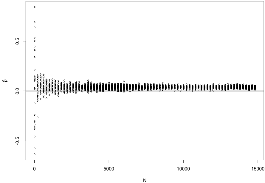
sim_cor = function(N = 10) {
  e = runif(N)
  x = (e - .5) + 100 * (e - .5)^2 + rnorm(N)
  cor(x, e)
}
Ns = rep(seq(10, 15000, 200), each = 30)
rs = numeric(length(Ns))
for (i in seq_along(Ns)) {
  rs[i] = sim_cor(Ns[i])
}
plot(Ns, rs, cex = .6, xlab = 'N', ylab = expression(hat(rho)))
abline(h = 0, lwd = 2)

Now I need to think why that is the case.

Originally posted on 2021-06-10 19:34:22

giscus-bot 2022-12-17 06:26:20

Guest *Eyayaw T. Beze* @ 2021-06-14 21:36:25 originally posted:

Thank you for the post. Find it very helpful.

giscus-bot 2022-12-17 06:26:21

Guest *jimrothstein* @ 2021-09-29 08:11:58 originally posted:

Learning a lot about OLS assumptions from this problem, though this post is still a bit over my head.

Some background reading I found, if useful to others.

Consistent Estimator: https://en.wikipedia.org/wiki/Consistent_estimator

Errors in predictor variables: https://en.wikipedia.org/wiki/Errors-in-variables_models

Ch 22 of this book by Norm Matloff:
http://heather.cs.ucdavis.edu/~matloff/132/PLN/probstatbook/ProbStatBook.pdf

Faraway has example of increasing the error in the predictor variable https://cran.r-project.org/doc/contrib/Faraway-PRA.pdf. He begins by assuming NO noise.

In this problem if the 'noise' is omitted, is it fair to create fake data as:

x = -1/2 + 25 * rnorm(N) # x is a RV  
y = 2*x + runif(N)